Ask
Questions provided by the case study
1-How do annual members and casual riders use Cyclistic bikes differently?
Problem Type: Business question
2-Why would casual riders buy Cyclistic annual memberships?
Problem Type: Business question
3-How can Cyclistic use digital media to influence casual riders to become members?
Problem Type: Business question
Prepare
Analyze with R.O.C.C.C
Reliability-The data is reliable as it consists of all the data of their users
Original-The data is from kaggle and it is the original data
Comprehensive-Yes the data is comprehensive
Current-The dataset is currect and containes data from 2020 to 2021
Cited-Yes
How are you addressing licensing, privacy, security, and accessibility?
The company has their own licence over the dataset. Besides that, the dataset doesn't have any personal information about the riders.
Process
Check the data for errors and transform the data to work with it effectively.
The data set given consisted of various .csv files but for this case study I have considered 12 csv files which contain the users data for each month
Installing Packages
  install.packages("tidyverse")
  install.packages("lubridate")
  install.packages("stringr")
  install.packages("scales")
  library(tidyverse)
  library(tidyr)
  library(dplyr)
  library(lubridate)
  library(stringr)
  library(scales)
  library(readr)
Converting the data to one datatype for merging the data
 m4_2020$start_station_id <- as.character(m4_2020$start_station_id)
 m4_2020$end_station_id <- as.character(m4_2020$end_station_id)
 m5_2020$end_station_id <- as.character(m5_2020$end_station_id)
 m5_2020$start_station_id <- as.character(m5_2020$start_station_id)
 m6_2020$start_station_id <- as.character(m6_2020$start_station_id)
 m6_2020$end_station_id <- as.character(m6_2020$end_station_id)
 m7_2020$end_station_id <- as.character(m7_2020$end_station_id)
 m7_2020$start_station_id <- as.character(m7_2020$start_station_id)
 m8_2020$start_station_id <- as.character(m8_2020$start_station_id)
 m8_2020$end_station_id <- as.character(m8_2020$end_station_id)
 m9_2020$end_station_id <- as.character(m9_2020$end_station_id)
 m9_2020$start_station_id <- as.character(m9_2020$start_station_id)
 m10_2020$start_station_id <- as.character(m10_2020$start_station_id)
 m10_2020$end_station_id <- as.character(m10_2020$end_station_id)
 m11_2020$end_station_id <- as.character(m11_2020$end_station_id)
 m11_2020$start_station_id <- as.character(m11_2020$start_station_id)
 m12_2020$start_station_id <- as.character(m12_2020$start_station_id)
 M12_2020$end_station_id <- as.character(M12_2020$end_station_id)
Merging the Data
 total <- full_join(m1_2021,m2_2021, by=c('ride_id','rideable_type','started_at', 'ended_at',"start_station_name","start_station_id","end_station_name","end_station_id","start_lat", "start_lng","end_lat","end_lng","member_casual"),copy=FALSE)
 total <- full_join(m1_2021,m2_2021, by=c('ride_id','rideable_type','started_at', 'ended_at',"start_station_name","start_station_id","end_station_name","end_station_id","start_lat", "start_lng","end_lat","end_lng","member_casual"),copy=FALSE)
 total <- full_join(total,m3_2021, by=c('ride_id','rideable_type','started_at', 'ended_at',"start_station_name","start_station_id","end_station_name","end_station_id","start_lat", "start_lng","end_lat","end_lng","member_casual"),copy=FALSE)
 total <- full_join(total,m4_2020, by=c('ride_id','rideable_type','started_at', 'ended_at',"start_station_name","start_station_id","end_station_name","end_station_id","start_lat", "start_lng","end_lat","end_lng","member_casual"),copy=FALSE)
 total <- full_join(total,m5_2020, by=c('ride_id','rideable_type','started_at', 'ended_at',"start_station_name","start_station_id","end_station_name","end_station_id","start_lat", "start_lng","end_lat","end_lng","member_casual"),copy=FALSE)
 total <- full_join(total,m6_2020, by=c('ride_id','rideable_type','started_at', 'ended_at',"start_station_name","start_station_id","end_station_name","end_station_id","start_lat", "start_lng","end_lat","end_lng","member_casual"),copy=FALSE)
 total <- full_join(total,m6_2020, by=c('ride_id','rideable_type','started_at', 'ended_at',"start_station_name","start_station_id","end_station_name","end_station_id","start_lat", "start_lng","end_lat","end_lng","member_casual"),copy=FALSE)
 total <- full_join(total,m7_2020, by=c('ride_id','rideable_type','started_at', 'ended_at',"start_station_name","start_station_id","end_station_name","end_station_id","start_lat", "start_lng","end_lat","end_lng","member_casual"),copy=FALSE)
 total <- full_join(total,m8_2020, by=c('ride_id','rideable_type','started_at', 'ended_at',"start_station_name","start_station_id","end_station_name","end_station_id","start_lat", "start_lng","end_lat","end_lng","member_casual"),copy=FALSE)
 total <- full_join(total,m9_2020, by=c('ride_id','rideable_type','started_at', 'ended_at',"start_station_name","start_station_id","end_station_name","end_station_id","start_lat", "start_lng","end_lat","end_lng","member_casual"),copy=FALSE)
 total <- full_join(total,m10_2020, by=c('ride_id','rideable_type','started_at', 'ended_at',"start_station_name","start_station_id","end_station_name","end_station_id","start_lat", "start_lng","end_lat","end_lng","member_casual"),copy=FALSE)
 total <- full_join(total,m11_2020, by=c('ride_id','rideable_type','started_at', 'ended_at',"start_station_name","start_station_id","end_station_name","end_station_id","start_lat", "start_lng","end_lat","end_lng","member_casual"),copy=FALSE)
 total <- full_join(total,M12_2020, by=c('ride_id','rideable_type','started_at', 'ended_at',"start_station_name","start_station_id","end_station_name","end_station_id","start_lat", "start_lng","end_lat","end_lng","member_casual"),copy=FALSE)
 final <-na.omit(total)
 final$Time <- format(final$started_at,"%H:%M:%S")
 final$eTime <- format(final$ended_at,"%H:%M:%S")
 final$eTime <- as.POSIXct(final$eTime,format="%H:%M:%S")
 final$Time <- as.POSIXct(final$Time,format="%H:%M:%S")
 View(final %>%
       + mutate(diff= difftime(eTime,Time, units = "mins")))
 final$diff <- difftime(final$ended_at,final$started_at, units = "mins")
Analyse
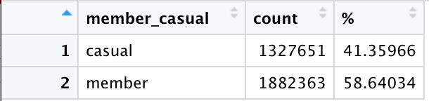
Casuals vs Members
    View(final %>%
    group_by(member_casual) %>%
    summarise(count = length(ride_id), '%' = (length(ride_id) / nrow(final)) * 100))
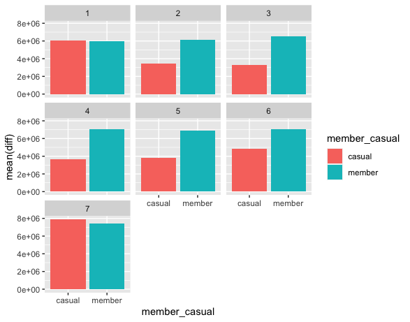
Amount of time Casual and Members use Cyclistic bikes in a week
        ggplot(data=final,mapping=aes(x=member_casual,y=mean(diff),fill=member_casual))+
        geom_bar(stat="identity")+
        facet_wrap(~wday(started_at))
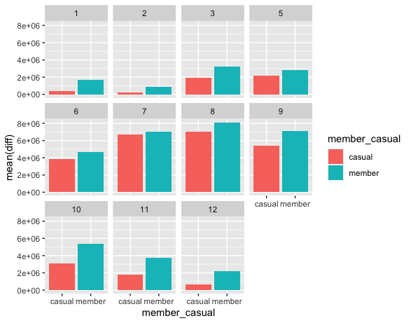
Amount of time Casual and Members use Cyclistic bikes per month
            ggplot(data=final,mapping=aes(x=member_casual,y=mean(diff),fill=member_casual))+
            geom_bar(stat="identity")+
            facet_wrap(~month(started_at))
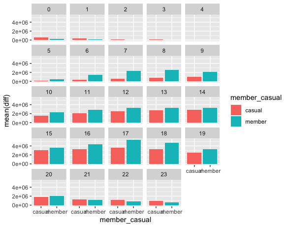
Amount of time Casual and Members use Cyclistic bikes per hour
                ggplot(data=final,mapping=aes(x=member_casual,y=mean(diff), fill=member_casual))+
                geom_bar(stat="identity")+
                facet_wrap( ~hour(started_at))
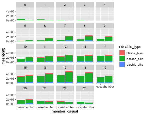
Amount of time Casual and Members use Cyclistic bikes per hour by Ride Type
                    ggplot(data=final,mapping=aes(x=member_casual,y=mean(diff), fill=member_casual))+
                    geom_bar(stat="identity")+
                    facet_wrap( ~hour(started_at))
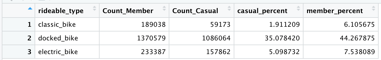
Types of Bikes members and non members use
                    View(final %>%
                    group_by(rideable_type) %>%
                    summarise(Count_Member= sum(member_casual=="member"),Count_Casual= sum(member_casual=="casual"),"casual_percent"=sum(member_casual=="casual")/nrow(final) *100 ,"member_percent"=sum(member_casual=="member")/nrow(final) *100))