Ask
Questions provided by the case study
1-What are some trends in smart device usage?
Problem Type: Making Predictions
2-How could these trends apply to Bellabeat customers?
Problem Type: Business question
3-How could these trends help influence Bellabeat marketing strategy?
Problem Type: Business question
Analysing question according to S.M.A.R.T
Specific-The given questions are not specific. There could be various trends that are irrelevant to the business.
Measurable-None of the questions asked have spoken about any measurable quantity.
Action-oriented- The trends required haven't been specified, hence there is no direction to this.
Relevant-There are missing quantities like 'age' and 'gender', hence some out the answers may not be specific.
Time-bound-The question's asked haven't stated any timeframe to calculate trends.
Prepare
Analyze with R.O.C.C.C
Reliability-The data were generated by respondents to a distributed survey via Amazon Mechanical Turk.
Original-No, the data was hosted by Mobius on Kaggle.
Comprehensive-No, the sample size is too small and fails to include perimeters like gender and age.
Current-No, the data is from 03/12/2016 - 05/12/2016.
Cited-Yes
Problems with the data
The data collected is out of date i.e.03/12/2016 - 05/12/2016.
The data is missing key arrtibutes such as age and gender.
Data set just include customers of FitBit Fitness Tracker, no other smart device users.
The database consist of just 33 users, hence it can not reflect the overall population
Process
Check the data for errors and transform the data to work with it effectively.
The data set given consisted of 18 .csv files consisting of heartrate, daily activity, hourly activity and every minute and second activity of 33 users which were in wide and long format
Installing Packages
  install.packages("tidyverse")
  install.packages("lubridate")
  install.packages("stringr")
  install.packages("scales")
  library(tidyverse)
  library(tidyr)
  library(dplyr)
  library(lubridate)
  library(stringr)
  library(scales)
  library(readr)
Working with dailyActivity, weight_new_weight and sleepDay_merged datasets
  dailyActivity_merged<- rename(dailyActivity_merged,"Date"="ActivityDate")
  activity_weight<- inner_join(dailyActivity_merged,weight_new_weightLogInfo_merged, by=c("Id","Date"))
  sleepDay_merged <- read_csv("~/Desktop/DA/Case Study 1/Fitabase Data 4.12.16-5.12.16/sleepDay_merged.csv")
  sleepDay_merged<- rename(sleepDay_merged,"Date"="SleepDay")
  sleepDay_merged$Date <- as.Date(sleepDay_merged$Date,"%m/%d/%Y")
  activity_weight<- inner_join(activity_weight,sleepDay_merged, by=c("Id","Date"))
  df = subset(activity_weight, select= -c(LoggedActivitiesDistance,Fat,TotalSleepRecords,TrackerDistance,
       VeryActiveDistance,ModeratelyActiveDistance,SedentaryActiveDistance,LightlyActiveMinutes,FairlyActiveMinutes,
       Date1,LightActiveDistance,VeryActiveMinutes,time,LogId))
  df<- arrange(df,TotalSteps)
Working with Hourly Data
  Hourly_df <-hourlyCalories_merged %>%
      + left_join(hourlyIntensities_merged, by= c('Id','ActivityHour')) %>%
      + left_join(hourlySteps_merged, by=c('Id','ActivityHour'))
  Hourly_df$DateTime <- head(mdy_hms(Hourly_df$ActivityHour, format = "%m/%d/%y %H:%M:%S %p"),-1)
  Hourly_df <- subset(Hourly_df,select=-ActivityHour)
Working with Minutely and Seconds Data
  Minutely_df <- minuteCaloriesWide_merged %>%
      +left_join(minuteIntensitiesWide_merged, by= c('Id','ActivityHour')) %>%
      +left_join(minuteStepsWide_merged, by=c('Id','ActivityHour'))
  heartrate_seconds_merged$DateTime <- head(mdy_hms(heartrate_seconds_merged$Time,
      format = "%m/%d/%y %H:%M:%S %p"),-1)
  heartrate_seconds_merged <- subset(heartrate_seconds_merged,select=-Time)
Analyse
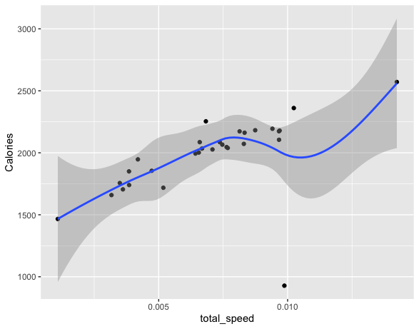
Relation between speed and calories
  activity_weight <- mutate(activity_weight, total_time_minutes=VeryActiveMinutes+ FairlyActiveMinutes +
     LightlyActiveMinutes + SedentaryMinutes)
  activity_weight <- mutate(activity_weight, total_speed= TotalDistance/ total_time_minutes)
  View(activity_weight)
  User <- filter(activity_weight,Id==6962181067)
  ggplot(data= User) +
    +geom_point(mapping=aes(x=total_speed, y=Calories))+
    + geom_smooth(mapping=aes(x=total_speed, y=Calories))
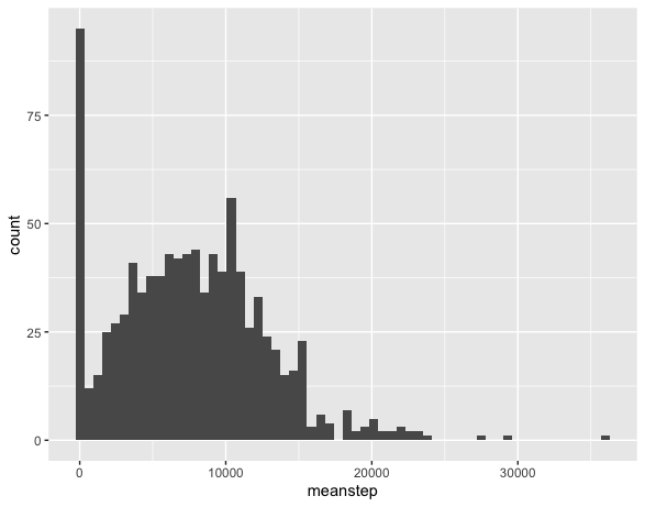
Mean steps per user
        dailyActivity_merged %>%
        + group_by(Id, Date) %>%
        + summarise(meanstep=mean(TotalSteps)) %>%
        + ggplot() +
        + geom_histogram(mapping=aes(x= meanstep),bins = 60)
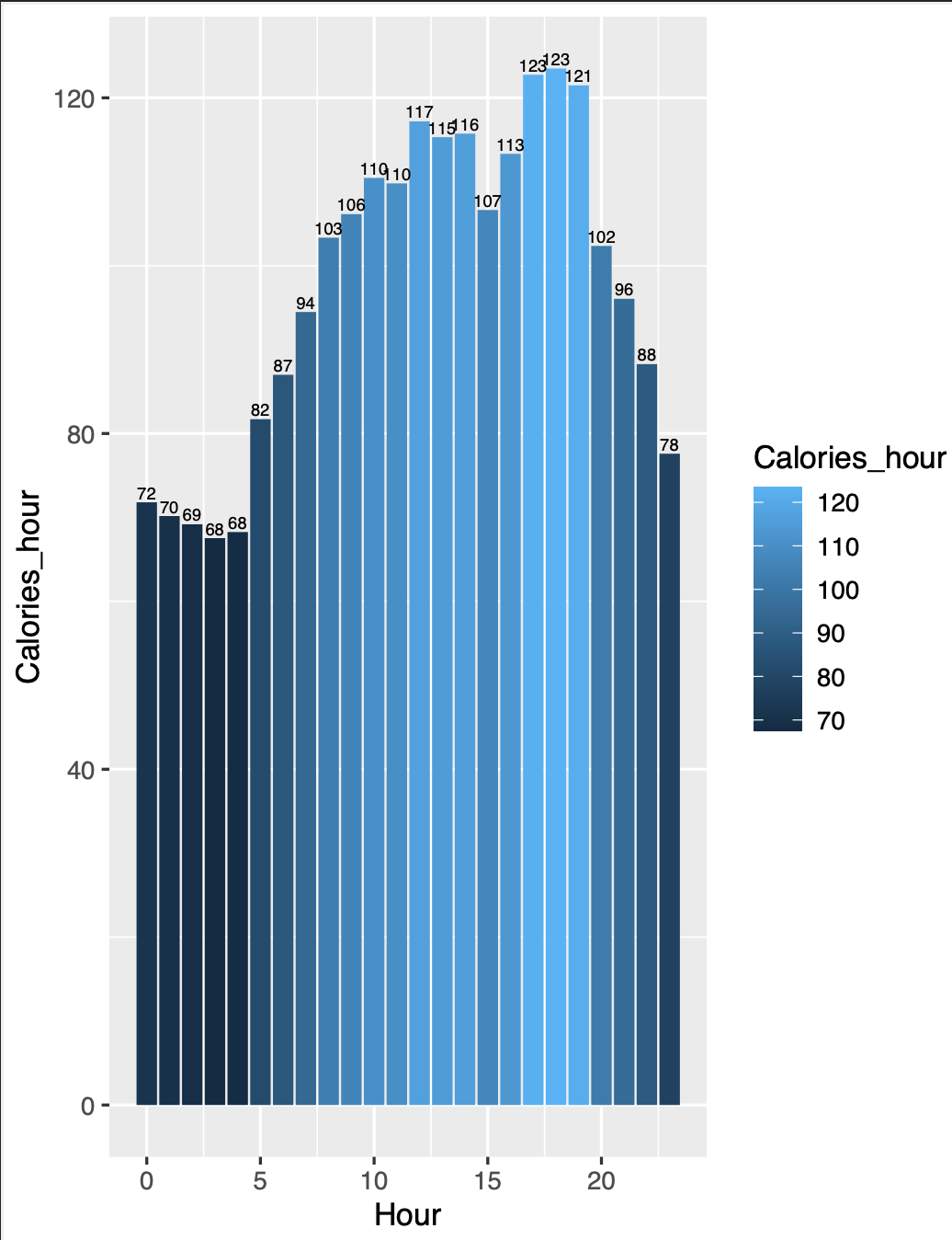
Calories consumed per hour
            Hourly_df %>%
            +     mutate(Hour=hour(DateTime)) %>%
            +     group_by(Hour) %>%
            +     summarise(Calories_hour=mean(Calories)) %>%
            +     ggplot(aes(x=Hour,y=Calories_hour,fill=Calories_hour))+
            +     geom_bar(stat="identity")+
            +     geom_text(aes(label=round(Calories_hour,0)), vjust=-0.3, size=2)
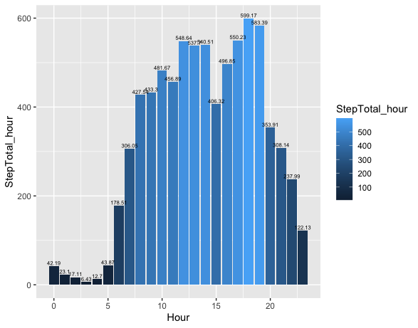
Total steps per hour
                Hourly_df %>%
                +     mutate(Hour=hour(DateTime)) %>%
                +     group_by(Hour) %>%
                +     summarise(StepTotal_hour=mean(StepTotal)) %>%
                +     ggplot(aes(x=Hour,y=StepTotal_hour,fill=StepTotal_hour))+
                +     geom_bar(stat="identity")+
                +     geom_text(aes(label=round(StepTotal_hour,2)), vjust=-0.3, size=2)
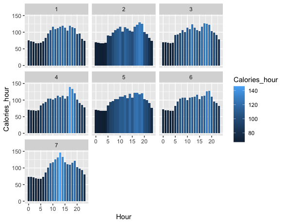
Calories consumed per hour each day
                    Hourly_df %>%
                    +     mutate(Hour=hour(DateTime),Day_of_week=wday(DateTime)) %>%
                    +     group_by(Day_of_week,Hour) %>%
                    +     summarise(Calories_hour=mean(Calories)) %>%
                    +     ggplot(aes(x=Hour,y=Calories_hour,fill=Calories_hour))+
                    +     geom_bar(stat="identity")+
                    +     facet_wrap(~Day_of_week)
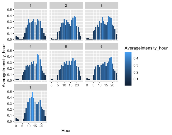
Intensity per hour each day
                        Hourly_df %>%
                        mutate(Hour=hour(DateTime),Day_of_week=wday(DateTime)) %>%
                        group_by(Day_of_week,Hour) %>%
                        summarise(AverageIntensity_hour=mean(AverageIntensity)) %>%
                        ggplot(aes(x=Hour,y=AverageIntensity_hour,fill=AverageIntensity_hour))+
                        geom_bar(stat="identity")+
                        facet_wrap(~Day_of_week)
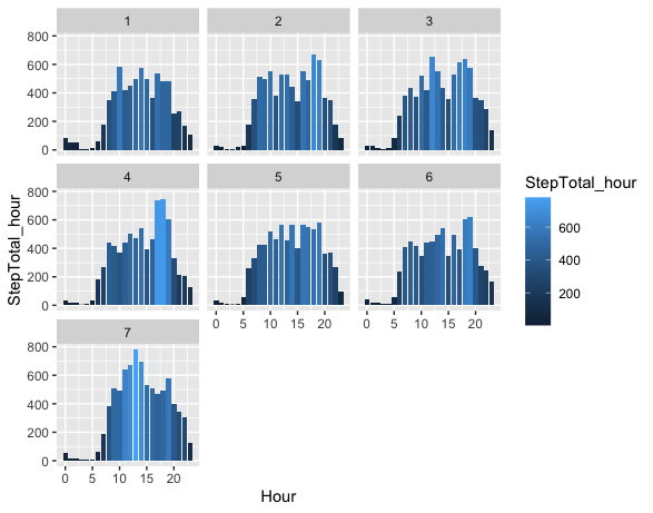
Total steps per hour each day
                            Hourly_df %>%
                            mutate(Hour=hour(DateTime),Day_of_week=wday(DateTime)) %>%
                            group_by(Day_of_week,Hour) %>%
                            summarise(StepTotal_hour=mean(StepTotal)) %>%
                            ggplot(aes(x=Hour,y=StepTotal_hour,fill=StepTotal_hour))+
                            geom_bar(stat="identity")+
                            facet_wrap(~Day_of_week)